
Homework 10: Neural Networks [100 points]
Instructions
In this assignment, you will implement functions commonly used in Neural Networks from scratch without use of external libraries/packages other than NumPy. Then, you will build Neural Networks using one of the Machine Learning frameworks called PyTorch for a Fashion MNIST dataset.
There are 2 skeleton files as listed at the top of the assignment. You should fill in your own code as suggested in this document. Since portions of this assignment will be graded automatically, none of the names or function signatures in this file should be modified. However, you are free to introduce additional variables or functions if needed.
You will find that in addition to a problem specification, most programming questions also include a pair of examples from the Python interpreter. These are meant to illustrate typical use cases, and should not be taken as comprehensive test suites.
You are strongly encouraged to follow the Python style guidelines set forth in PEP 8, which was written in part by the creator of Python. However, your code will not be graded for style.
Once you have finished the assignment, you should submit both 2 completed skeleton files on Gradescope. You may submit as many times as you would like before the deadline, but only the last submission will be saved.
Here are some for this assignment:
- Numpy is very useful for the CNN functions part of the assignment. For the convolve_grayscale function, the following numpy commands might be useful:
- numpy.fliplr and numpy.flipud - useful for flipping the kernel
- numpy.shape - can be used to get the dimensions of a numpy array like the image or the kernel. For example: image_height, image_width = image.shape & numpy.zeros - useful for imitating the output to be the size of the image_height, image_width
- numpy.hstack and numpy.vstack - useful for padding the image
- numpy.arange - useful for looping over the image. For example:
for y in np.arange(vertical_pad, image_height + vertical_pad): for x in np.arange(horizontal_pad, image_width + horizontal_pad): output[y - vertical_pad, x - horizontal_pad] = // your code here - numpy.sum - useful for summing over the values in an array (hint: will simplify the “your code here” above)
- Hint: After you’ve implemented convolve_grayscale, your convolve_rgb function can by very short. All you have to do is to call your convolve_grayscale three times - once for the red channel, once for the green channel and once for the blue channel. The slice notation from early in the course will also be very useful.
output[:, :, channel] = // your code here - For your max_pooling and your average_pooling functions:
- numpy.lib.stride_tricks.as_strided - is useful for both. Here is a nice illustrated tutoral on how to use stride tricks.
- numpy.mean - useful for mean_pooling
- numpy.maximum - useful for max_pooling
-
PyTorch is very useful for defining your models for the Fashion MNIST part of the assignment. I recommend taking the time to walk through a tutorial on how to use it. This tutorial uses the Fashion MNIST data set, and we based the assignment on parts on the tutorial.
- Here’s some documentation that for PyTorch that are used in the assignment:
- torch.nn.Linear
- torch.nn.ReLU - use to compute the rectified linear unit activation function
- torch.nn.LogSoftmax - softmax
- torch.nn.Conv2d - use in the advanced model
- torch.nn.BatchNorm2d - use in the advanced model
- torch.nn.MaxPool2d- use in the advanced model
1. Individual Functions for CNN [50 points]
The goal of this part of the assignment is to get an intuition of the underlying implementation used in Convolutional Neural Networks (CNN), specifically performing convolution and pooling, and applying an activation function.
As mentioned in the instructions, you are restricted from using any external packages other than NumPy. Numpy has a Quickstart tutorial, which we recommend looking at if you are not familiar or would like to refresh memory.
-
[18 points] Write a function
convolve_greyscale(image, kernel)that accepts a numpy arrayimageof shape(image_height, image_width)(greyscale image) of integers and a numpy arraykernelof shape(kernel_height, kernel_width)of floats. The function performs a convolution, which consists of adding each element of the image to its local neighbors, weighted by the kernel (flipped both vertically and horizontally).The result of this function is a new numpy array of floats that has the same shape as the input
image. Apply zero-padding to the input image to calculate image edges. Note that the height and width of bothimageandkernelmight not be equal to each other. You can assumekernel_widthandkernel_heightare odd numbers.There exist a few visualisations hands-on experience of applying a convolution online, for instance a post by Victor Powell. For more information, you can also use real images as an input. We recommend selecting a few images of type
grayfrom the Miscellaneous Volume of the USC-SIPI Image Database. (Image in the third example below is taken from this dataset labelled under 5.1.09.)>>> import numpy as np >>> image = np.array([ [0, 1, 2, 3, 4], [ 5, 6, 7, 8, 9], [10, 11, 12, 13, 14], [15, 16, 17, 18, 19], [20, 21, 22, 23, 24]]) >>> kernel = np.array([ [0, -1, 0], [-1, 5, -1], [0, -1, 0]]) >>> print(convolve_greyscale(image, kernel)) [[-6. -3. -1. 1. 8.] [ 9. 6. 7. 8. 19.] [19. 11. 12. 13. 29.] [29. 16. 17. 18. 39.] [64. 47. 49. 51. 78.]]>>> import numpy as np >>> image = np.array([ [0, 1, 2, 3, 4], [ 5, 6, 7, 8, 9], [10, 11, 12, 13, 14], [15, 16, 17, 18, 19], [20, 21, 22, 23, 24]]) >>> kernel = np.array([ [1, 2, 3], [0, 0, 0], [-1, -2, -3]]) >>> print(convolve_greyscale(image, kernel)) [[ 16. 34. 40. 46. 42.] [ 30. 60. 60. 60. 50.] [ 30. 60. 60. 60. 50.] [ 30. 60. 60. 60. 50.] [ -46. -94. -100. -106. -92.]]>>> import numpy as np >>> from PIL import Image >>> import matplotlib.pyplot as plt >>> image = np.array(Image.open('5.1.09.tiff')) >>> plt.imshow(image, cmap='gray') >>> plt.show() >>> kernel = np.array([ [0, -1, 0], [-1, 5, -1], [0, -1, 0]]) >>> output = convolve_greyscale(image, kernel) >>> plt.imshow(output, cmap='gray') >>> plt.show() >>> print(output) [[416. 352. 270. ... 152. 135. 233.] [274. 201. 126. ... 85. 69. 155.] [255. 151. 131. ... 56. 45. 164.] ... [274. 124. 159. ... 91. 176. 241.] [166. 139. 118. ... 122. 156. 280.] [423. 262. 280. ... 262. 312. 454.]]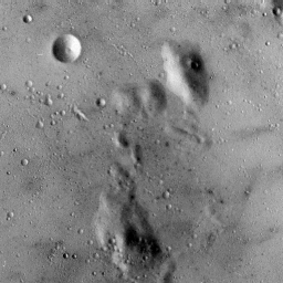
Left: line 6 (before function invocation)
Right: line 10 (after function invocation) -
[4 points] Write a function
convolve_rgb(image, kernel)that accepts a numpy arrayimageof shape(image_height, image_width, image_depth)of integers and a numpy arraykernelof shape(kernel_height, kernel_width)of floats. The function performs a convolution on each depth of an image, which consists of adding each element of the image to its local neighbors, weighted by the kernel (flipped both vertically and horizontally).The result of this function is a new numpy array of floats that has the same shape as the input
image. You can useconvolve_greyscale(image, filter)implemented in the previous part to go through each depth of an image. As before, apply zero-padding to the input image to calculate image edges. Note that the height and width of bothimageandkernelmight not be equal to each other. You can assumekernel_widthandkernel_heightare odd numbers.We recommend selecting a few images of type
colorfrom the Miscellaneous Volume of the USC-SIPI Image Database. (Images in the examples below are taken from this dataset labelled under 4.1.07)>>> import numpy as np >>> from PIL import Image >>> import matplotlib.pyplot as plt >>> image = np.array(Image.open('4.1.07.tiff')) >>> plt.imshow(image) >>> plt.show() >>> kernel = np.array([ [0.11111111, 0.11111111, 0.11111111], [0.11111111, 0.11111111, 0.11111111], [0.11111111, 0.11111111, 0.11111111]]) >>> output = convolve_rgb(image, kernel) >>> plt.imshow(output.astype('uint8')) >>> plt.show() >>> print(np.round(output[0:3, 0:3, 0:3], 2)) [[[ 63.67 63.44 47.22] [ 95.56 94.89 70.89] [ 95.56 94.78 70.89]] [[ 95.67 95.22 70.67] [143.33 142.56 105.89] [143.22 142.33 106. ]] [[ 96.33 96.11 70.22] [144.11 144. 105.11] [143.78 143.44 105.22]]]
Left: line 6 (before function invocation)
Right: line 10 (after function invocation)>>> import numpy as np >>> from PIL import Image >>> import matplotlib.pyplot as plt >>> image = np.array(Image.open('4.1.07.tiff')) >>> plt.imshow(image) >>> plt.show() >>> kernel = np.ones((11, 11)) >>> kernel /= np.sum(kernel) >>> output = convolve_rgb(image, kernel) >>> plt.imshow(output.astype('uint8')) >>> plt.show() >>> print(np.round(output[0:3, 0:3, 0:3], 2)) [[[43.26 43.31 31.32] [50.54 50.67 36.6 ] [57.83 58. 41.88]] [[50.64 50.86 36.51] [59.17 59.5 42.65] [67.73 68.1 48.81]] [[58.01 58.49 41.7 ] [67.79 68.41 48.72] [77.6 78.29 55.75]]] Left: line 6 (before function invocation)
Right: line 11 (after function invocation) -
[20 points] Write a function
max_pooling(image, kernel_size, stride)that accepts a numpy arrayimageof integers of shape(image_height, image_width)(greyscale image) of integers, a tuplekernel_sizecorresponding to(kernel_height, kernel_width), and a tuplestrideof(stride_height, stride_width)corresponding to the stride of pooling window.The goal of this function is to reduce the spatial size of the representation and in this case reduce dimensionality of an image with max down-sampling. It is not common to pad the input using zero-padding for the pooling layer in Convolutional Neural Network and as such, so we do not ask to pad. Notice that this function must support overlapping pooling if
strideis not equal tokernel_size.As before, we recommend selecting a few images of type
grayfrom the Miscellaneous Volume of the USC-SIPI Image Database. (Image in three examples below are taken from this dataset labelled under 5.1.09.)>>> image = np.array([ [1, 1, 2, 4], [5, 6, 7, 8], [3, 2, 1, 0], [1, 2, 3, 4]]) >>> kernel_size = (2, 2) >>> stride = (2, 2) >>> print(max_pooling(image, kernel_size, stride)) [[6 8] [3 4]]>>> image = np.array([ [1, 1, 2, 4], [5, 6, 7, 8], [3, 2, 1, 0], [1, 2, 3, 4]]) >>> kernel_size = (2, 2) >>> stride = (1, 1) >>> print(max_pooling(image, kernel_size, stride)) [[6 7 8] [6 7 8] [3 3 4]]>>> import numpy as np >>> from PIL import Image >>> import matplotlib.pyplot as plt >>> image = np.array(Image.open('5.1.09.tiff')) >>> plt.imshow(image, cmap='gray') >>> plt.show() >>> kernel_size = (2, 2) >>> stride = (2, 2) >>> output = max_pooling(image, kernel_size, stride) >>> plt.imshow(output, cmap='gray') >>> plt.show() >>> print(output) [[160 146 155 ... 73 73 76] [160 148 153 ... 75 73 84] [168 155 155 ... 80 66 80] ... [137 133 131 ... 148 149 146] [133 133 129 ... 146 144 146] [133 133 133 ... 151 148 149]] >>> print(output.shape) (128, 128) Left: line 6 (before function invocation with image shape (256, 256))
Right: line 11 (after function invocation with image shape (128, 128))>>> import numpy as np >>> from PIL import Image >>> import matplotlib.pyplot as plt >>> image = np.array(Image.open('5.1.09.tiff')) >>> plt.imshow(image, cmap='gray') >>> plt.show() >>> kernel_size = (4, 4) >>> stride = (1, 1) >>> output = max_pooling(image, kernel_size, stride) >>> plt.imshow(output, cmap='gray') >>> plt.show() >>> print(output) [[160 160 155 ... 75 73 84] [162 160 155 ... 80 76 84] [168 168 155 ... 80 76 84] ... [137 133 133 ... 149 149 149] [133 133 133 ... 149 149 149] [133 133 133 ... 151 149 149]] >>> print(output.shape) (253, 253) Left: line 6 (before function invocation with image shape (256, 256))
Right: line 11 (after function invocation with image shape (253, 253))>>> import numpy as np >>> from PIL import Image >>> import matplotlib.pyplot as plt >>> image = np.array(Image.open('5.1.09.tiff')) >>> plt.imshow(image, cmap='gray') >>> plt.show() >>> kernel_size = (3, 3) >>> stride = (1, 3) >>> output = max_pooling(image, kernel_size, stride) >>> plt.imshow(output, cmap='gray') >>> plt.show() >>> print(output) [[160 155 153 ... 100 76 73] [160 155 153 ... 113 82 73] [162 155 157 ... 118 82 76] ... [133 133 126 ... 155 148 149] [133 133 131 ... 149 148 148] [133 133 131 ... 146 151 149]] >>> print(output.shape) (254, 85) Left: line 6 (before function invocation with image shape (256, 256))
Right: line 11 (after function invocation with image shape (254, 85)) -
[4 points] Similarly to the previous part, write a function
average_pooling(image, kernel_size, stride)that accepts a numpy arrayimageof integers of shape(image_height, image_width)(greyscale image) of integers, a tuplekernel_sizecorresponding to(kernel_height, kernel_width), and a tuplestrideof(stride_height, stride_width)corresponding to the stride of pooling window.The goal of this function is to reduce the spatial size of the representation and in this case reduce dimensionality of an image with average down-sampling.
As before, we recommend selecting a few images of type
grayfrom the Miscellaneous Volume of the USC-SIPI Image Database. (Image in the third example is taken from this dataset labelled under 5.1.09.)>>> image = np.array([ [1, 1, 2, 4], [5, 6, 7, 8], [3, 2, 1, 0], [1, 2, 3, 4]]) >>> kernel_size = (2, 2) >>> stride = (2, 2) >>> print(average_pooling(image, kernel_size, stride)) [[3.25 5.25] [2. 2. ]]>>> image = np.array([ [1, 1, 2, 4], [5, 6, 7, 8], [3, 2, 1, 0], [1, 2, 3, 4]]) >>> kernel_size = (2, 2) >>> stride = (1, 1) >>> print(average_pooling(image, kernel_size, stride)) [[3.25 4. 5.25] [4. 4. 4. ] [2. 2. 2. ]]>>> import numpy as np >>> from PIL import Image >>> import matplotlib.pyplot as plt >>> image = np.array(Image.open('5.1.09.tiff')) >>> plt.imshow(image, cmap='gray') >>> plt.show() >>> kernel_size = (2, 2) >>> stride = (2, 2) >>> output = average_pooling(image, kernel_size, stride) >>> plt.imshow(output, cmap='gray') >>> plt.show() >>> print(output) [[152. 145. 154. ... 65.5 71. 73.5 ] [152.75 145.5 143.25 ... 70.5 68.25 74.25] [160.5 149.5 146.25 ... 71. 62.25 75. ] ... [129. 128.75 125.25 ... 144. 138.25 141.75] [127.75 128. 125. ... 142. 135.75 142.25] [125.5 127.75 130. ... 143.75 141.25 146.5 ]] >>> print(output.shape) (128, 128) Left: line 6 (before function invocation with image shape (256, 256))
Right: line 11 (after function invocation with image shape (128, 128))>>> import numpy as np >>> from PIL import Image >>> import matplotlib.pyplot as plt >>> image = np.array(Image.open('5.1.09.tiff')) >>> plt.imshow(image, cmap='gray') >>> plt.show() >>> kernel_size = (4, 4) >>> stride = (1, 1) >>> output = average_pooling(image, kernel_size, stride) >>> plt.imshow(output, cmap='gray') >>> plt.show() >>> print(output) [[148.8125 149.375 146.9375 ... 68.8125 69.875 71.75 ] [149.5 148. 145.625 ... 69.4375 69.4375 71. ] [152.0625 149. 146.125 ... 68. 67.4375 69.9375] ... [128.375 127. 126.75 ... 140. 139.6875 139.5 ] [126.625 127. 127.1875 ... 140.75 140.9375 140.5 ] [127.25 127.8125 127.6875 ... 140.6875 141.0625 141.4375]] >>> print(output.shape) (253, 253) Left: line 6 (before function invocation with image shape (256, 256))
Right: line 11 (after function invocation with image shape (253, 253))>>> import numpy as np >>> from PIL import Image >>> import matplotlib.pyplot as plt >>> image = np.array(Image.open('5.1.09.tiff')) >>> plt.imshow(image, cmap='gray') >>> plt.show() >>> kernel_size = (3, 3) >>> stride = (1, 3) >>> output = average_pooling(image, kernel_size, stride) >>> plt.imshow(output, cmap='gray') >>> plt.show() >>> print(np.round(output, 5)) [[148.11111 150.88889 149.33333 ... 79.33333 66.66667 69.55556] [150.11111 146.33333 147.55556 ... 85. 70.33333 69. ] [150.33333 144.44444 146.55556 ... 93.44444 73.55556 68.22222] ... [127.88889 125.55556 118.66667 ... 146. 142.22222 138.66667] [126.11111 126.55556 123.77778 ... 143.66667 142.44444 140.22222] [127.88889 128.11111 125.88889 ... 142.88889 143.55556 141.55556]] >>> print(output.shape) (254, 85) Left: line 6 (before function invocation with image shape (256, 256))
Right: line 11 (after function invocation with image shape (254, 85)) -
[4 points] Write a function
sigmoid(x)that accepts an a numpy arrayxand applies a sigmoid activation function on the input.>>> x = np.array([0.5, 3, 1.5, -4.7, -100]) >>> print(sigmoid(x)) [6.22459331e-01 9.52574127e-01 8.17574476e-01 9.01329865e-03 3.72007598e-44]
2. Neural Network for Fashion MNIST Dataset [45 points]
The goal of this part of the assignment is to get familiar with using one of the Machine Learning frameworks called PyTorch.
The installation instructions can be found here. If you are having difficulty installing it, here is an alternative way to setup PyTorch using miniconda.
(Setup PyTorch using miniconda)
Miniconda is a package, dependency and environment management for python (amongst other languages). It lets you install different versions of python, different versions of various packages in different environments which makes working on multiple projects (with different dependencies) easy.
There are two ways to use miniconda,
- Use an existing installation from another user (highly recommended): On
biglab, add the following line at the end of your~/.bashrcfile.export PATH="/home1/m/mayhew/miniconda3/bin:$PATH"Then run the following command
source ~/.bashrcIf you run the command
$ which conda, the output should be/home1/m/mayhew/miniconda3/bin/conda. - Installing Miniconda from scratch: On
biglab, run the following commands. Press Enter/Agree to all prompts during installation.$ wget https://repo.continuum.io/miniconda/Miniconda3-latest-Linux-x86_64.sh $ chmod +x Miniconda3-latest-Linux-x86_64.sh $ bash Miniconda3-latest-Linux-x86_64.shAfter successful installation, running the command
$ which condashould output/home1/m/$USERNAME/miniconda3/bin/conda.
Fashion MNIST Dataset
The dataset.csv we will use is a sub-set of the Fashion MNIST train dataset.
![]()
The dataset contains 20000 28x28 greyscale images, where each image has a label from one of 10 classes:
| Label | Description |
|---|---|
| 0 | T-shirt/top |
| 1 | Trouser |
| 2 | Pullover |
| 3 | Dress |
| 4 | Coat |
| 5 | Sandal |
| 6 | Shirt |
| 7 | Sneaker |
| 8 | Bag |
| 9 | Ankle boot |
-
[5 points] The dataset.csv is a comma-separated csv file with a header ‘label, pixel1, pixel2, …, pixel 784’. The first column ‘label’ is a label from 0 to 9 inclusively, and the rest of the columns ‘pixel1’ … ‘pixel784’ are 784 pixels of an image for a corresponding label.
Your task is to fill in
load_data(file_path, reshape_images), wherefile_pathis a string representing the path to a dataset andreshape_imagesis a boolean flag that indicates whether an image needs to be represented as one dimensional array of 784 pixels or reshaped to (1, 28, 28) array pixels. This function returns 2 numpy arrays, where the first array corresponds to images and the second to labels.Since there are 20000 images and labels in
dataset.csv, you should expect something as follows when the function is called withreshape_imagesset toFalse:>>> X, Y = load_data('dataset.csv', False) >>> print(X.shape) (20000, 784) >>> print(Y.shape) (20000,)And something as follows when the function is called with
reshape_imagesset toTrue:>>> X, Y = load_data('dataset.csv', True) >>> print(X.shape) (20000, 1, 28, 28) >>> print(Y.shape) (20000,)Here is a way to visualise the first image of our data:
 >>> import matplotlib.pyplot as plt
 >>> class_names = ['T-Shirt', 'Trouser', 'Pullover', 'Dress', 'Coat', 'Sandal', 'Shirt', 'Sneaker', 'Bag', 'Ankle Boot']
 >>> X, Y = load_data('dataset.csv', False)
 >>> plt.imshow(X[0].reshape(28, 28), cmap='gray')
 >>> plt.title(class_names[Y[0]])
 >>> plt.show()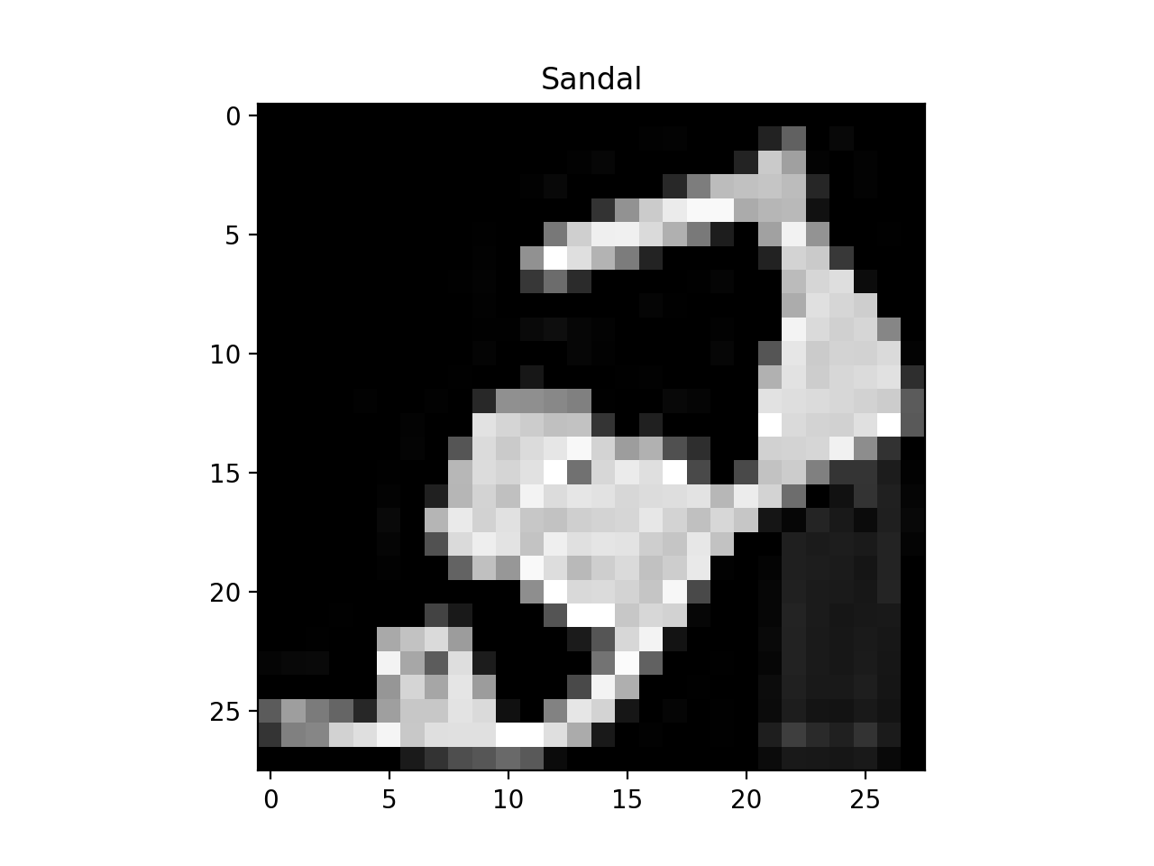
Data Loading and Processing in PyTorch
The
load_data(file_path, reshape_images)function gets called in theFashionMNISTDatasetclass, which is given in the skeleton file. TheFashionMNISTDatasetclass is a custom dataset that inheritstorch.utils.data.Dataset, which is an abstract class representing a dataset in PyTorch. We filled in the required__len__and__getitem__functions to return the size of the dataset and to add support the indexing of the dataset.from torch.utils.data import Dataset class FashionMNISTDataset(Dataset): def __init__(self, file_path, reshape_images): self.X, self.Y = load_data(file_path, reshape_images) def __len__(self): return len(self.X) def __getitem__(self, index): return self.X[index], self.Y[index]Similarly to the previous snippets of code:
 >>> dataset= FashionMNISTDataset('dataset.csv', False)
 >>> print(dataset.X.shape)
 (20000, 784)
 >>> print(dataset.Y.shape)
 (20000,)
 >>> dataset= FashionMNISTDataset('dataset.csv', True)
 >>> print(dataset.X.shape)
 (20000, 1, 28, 28)
 >>> print(dataset.Y.shape)
 (20000,)
This
FashionMNISTDatasetclass can be used bytorch.utils.data.DataLoader, which is a dataset iterator and that provides ways to batch the data, shuffle the data, or load the data in parallel. Here is a snippet of code that usestorch.utils.data.DataLoaderwithbatch_sizeset to 10:>>> dataset = FashionMNISTDataset('dataset.csv', False) >>> data_loader = torch.utils.data.DataLoader(dataset=dataset, batch_size=10, shuffle=False) >>> print(len(data_loader)) 2000 >>> images, labels = list(data_loader)[0] >>> print(type(images)) <class torch.LongTensor> >>> print(images) <class torch.LongTensor> 0 0 0 ... 25 9 0 0 0 0 ... 0 0 0 0 0 0 ... 0 0 0 ... ... ... 0 0 0 ... 0 0 0 0 0 0 ... 0 0 0 0 0 1 ... 0 0 0 [torch.LongTensor of size 10x784] >>> print(type(labels)) <class torch.LongTensor> >>> print(labels) 5 0 1 4 7 6 2 1 9 0 [torch.LongTensor of size 10]Note that we added the code to load the data with
torch.utils.data.DataLoaderin themain()function of the skeleton file. -
[40 points] For the next part of the assignment we give you a few functions that you are welcome to use and modify. They are:
- The
train(model, data_loader, num_epochs, learning_rate)function, which accepts the following arguments- a
modelwhich is a subclass oftorch.nn.Module, - a
data_loaderwhich is a class oftorch.utils.data.DataLoader - two hyper-parameters:
num_epochsandlearning_rate. This function trains amodelfor the specifiednum_epochsusingtorch.nn.CrossEntropyLossloss function andtorch.optim.Adamas an optimizer. Once in a specified amount of iterations, the function prints the current loss, train accuracy, train F1-score for the model.
- a
- The
evaluate(model, data_loader)function, which accepts- a
modelwhich is a subclass oftorch.nn.Module - a
data_loaderwhich is a class oftorch.utils.data.DataLoader.
The
evaluatefunction returns a list of actual labels and a list of predicted labels by thatmodelfor thisdata_loaderclass. This function can be used to get the metrics, such as accuracy or F1-score. - a
- The
plot_confusion_matrix(cm, class_names, title=None)function, which visualises a confusion matrix. It accepts- a confusion matrix
cm, - a list of corresponding
class_names - an optional
title.
The
plot_confusion_matrixfunction was modified from here. - a confusion matrix
All you have to do is to fill in
__init__(self)andforward(self, x)for 3 different classes: Easy, Medium, and Advanced.-
[10 pts] Easy Model: In this part we ask you to fill in
__init__(self)andforward(self, x)of theEasyModelclass.EasyModelis a subclass oftorch.nn.Module, which is a base class for all neural network models in PyTorch. We ask you to build a model that consists of a single linear layer (usingtorch.nn.Linear). You will need to write one line of code. It starts withself.fc = torch.nn.Linear. It maps the size of the representation of an image to the number of classes. We recommend to have look around the API fortorch.nn.Once you have filled in
__init__(self)andforward(self, x)of theEasyModelclass you should expect something similar to this:>>> class_names = ['T-Shirt', 'Trouser', 'Pullover', 'Dress', 'Coat', 'Sandal', 'Shirt', 'Sneaker', 'Bag', 'Ankle Boot'] >>> num_epochs = 2 >>> batch_size = 100 >>> learning_rate = 0.001 >>> data_loader = torch.utils.data.DataLoader(dataset=FashionMNISTDataset('dataset.csv', False), batch_size=batch_size, shuffle=True) >>> easy_model = EasyModel() >>> train(easy_model, data_loader, num_epochs, learning_rate) Epoch : 0/2, Iteration : 49/200, Loss: 5.7422, Train Accuracy: 73.3450, Train F1 Score: 72.6777 Epoch : 0/2, Iteration : 99/200, Loss: 7.6222, Train Accuracy: 76.7650, Train F1 Score: 75.8522 Epoch : 0/2, Iteration : 149/200, Loss: 8.9238, Train Accuracy: 76.9600, Train F1 Score: 76.6251 Epoch : 0/2, Iteration : 199/200, Loss: 6.3722, Train Accuracy: 76.9450, Train F1 Score: 77.1084 Epoch : 1/2, Iteration : 49/200, Loss: 6.0220, Train Accuracy: 72.7300, Train F1 Score: 73.4246 Epoch : 1/2, Iteration : 99/200, Loss: 4.4724, Train Accuracy: 78.5450, Train F1 Score: 78.6831 Epoch : 1/2, Iteration : 149/200, Loss: 3.9865, Train Accuracy: 79.5950, Train F1 Score: 79.3139 Epoch : 1/2, Iteration : 199/200, Loss: 4.8550, Train Accuracy: 75.4150, Train F1 Score: 73.7432 >>> y_true_easy, y_pred_easy = evaluate(easy_model, data_loader) >>> print(f'Easy Model: ' f'Final Train Accuracy: {100.* accuracy_score(y_true_easy, y_pred_easy):.4f},', f'Final Train F1 Score: {100.* f1_score(y_true_easy, y_pred_easy, average="weighted"):.4f}') Easy Model: Final Train Accuracy: 75.4150, Final Train F1 Score: 73.7432 >>> plot_confusion_matrix(confusion_matrix(y_true_easy, y_pred_easy), class_names, 'Easy Model')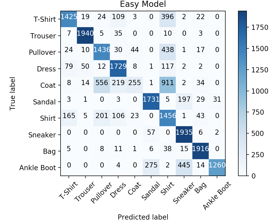
We reserved multiple datasets for testing with the same distribution of labels as given in
dataset.csv. We will train and evaluate your model on our end using the sametrain()andevaluate()functions as given. Full points will be given for anEasy Modelfor num_epochs = 2, batch_size = 100, learning_rate = 0.001 if the accuracy on the reserved datasets and F1-Score is >= 73%. -
[15 pts] Medium Model: In this part we ask you to fill in
__init__(self)andforward(self, x)of theMediumModelclass that is a subclass oftorch.nn.Module. We ask you to build a model that consists of a multiple fully-connected linear layers (usingtorch.nn.Linear). The network architecture is open-ended, so it is up to you to decide the number of linear layers and the size of nodes within the hidden layer(s). There are many tutorials online for you to use, for instance this blog post gives a good solution for ourMediumclass by building a Fully-Connected Network with 2 hidden layers. You can also use activation functions like ReLU. Remember that the input to this model is the size of a one dimensional representation of an image and the output is the number of classes as for the Easy Model.Once you have filled in
__init__(self)andforward(self, x)of theMediumModelclass you should expect something similar to this:>>> class_names = ['T-Shirt', 'Trouser', 'Pullover', 'Dress', 'Coat', 'Sandal', 'Shirt', 'Sneaker', 'Bag', 'Ankle Boot'] >>> num_epochs = 2 >>> batch_size = 100 >>> learning_rate = 0.001 >>> data_loader = torch.utils.data.DataLoader(dataset=FashionMNISTDataset('dataset.csv', False), batch_size=batch_size, shuffle=True) >>> medium_model = MediumModel() >>> train(medium_model, data_loader, num_epochs, learning_rate) >>> y_true_medium, y_pred_medium = evaluate(medium_model, data_loader) Epoch : 0/2, Iteration : 49/200, Loss: 0.7257, Train Accuracy: 76.7000, Train F1 Score: 76.6240 Epoch : 0/2, Iteration : 99/200, Loss: 0.6099, Train Accuracy: 79.6000, Train F1 Score: 79.3427 Epoch : 0/2, Iteration : 149/200, Loss: 0.3406, Train Accuracy: 80.3550, Train F1 Score: 79.2653 Epoch : 0/2, Iteration : 199/200, Loss: 0.4423, Train Accuracy: 82.2350, Train F1 Score: 82.1259 Epoch : 1/2, Iteration : 49/200, Loss: 0.6591, Train Accuracy: 82.2450, Train F1 Score: 81.5656 Epoch : 1/2, Iteration : 99/200, Loss: 0.5055, Train Accuracy: 81.7150, Train F1 Score: 81.2029 Epoch : 1/2, Iteration : 149/200, Loss: 0.4616, Train Accuracy: 83.9600, Train F1 Score: 83.4397 Epoch : 1/2, Iteration : 199/200, Loss: 0.3895, Train Accuracy: 84.3500, Train F1 Score: 84.3794 >>> print(f'Medium Model: ' f'Final Train Accuracy: {100.* accuracy_score(y_true_medium, y_pred_medium):.4f},', f'Final F1 Score: {100.* f1_score(y_true_medium, y_pred_medium, average="weighted"):.4f}') Medium Model: Final Train Accuracy: 84.3500, Final F1 Score: 84.3794 >>> plot_confusion_matrix(confusion_matrix(y_true_medium, y_pred_medium), class_names, 'Medium Model')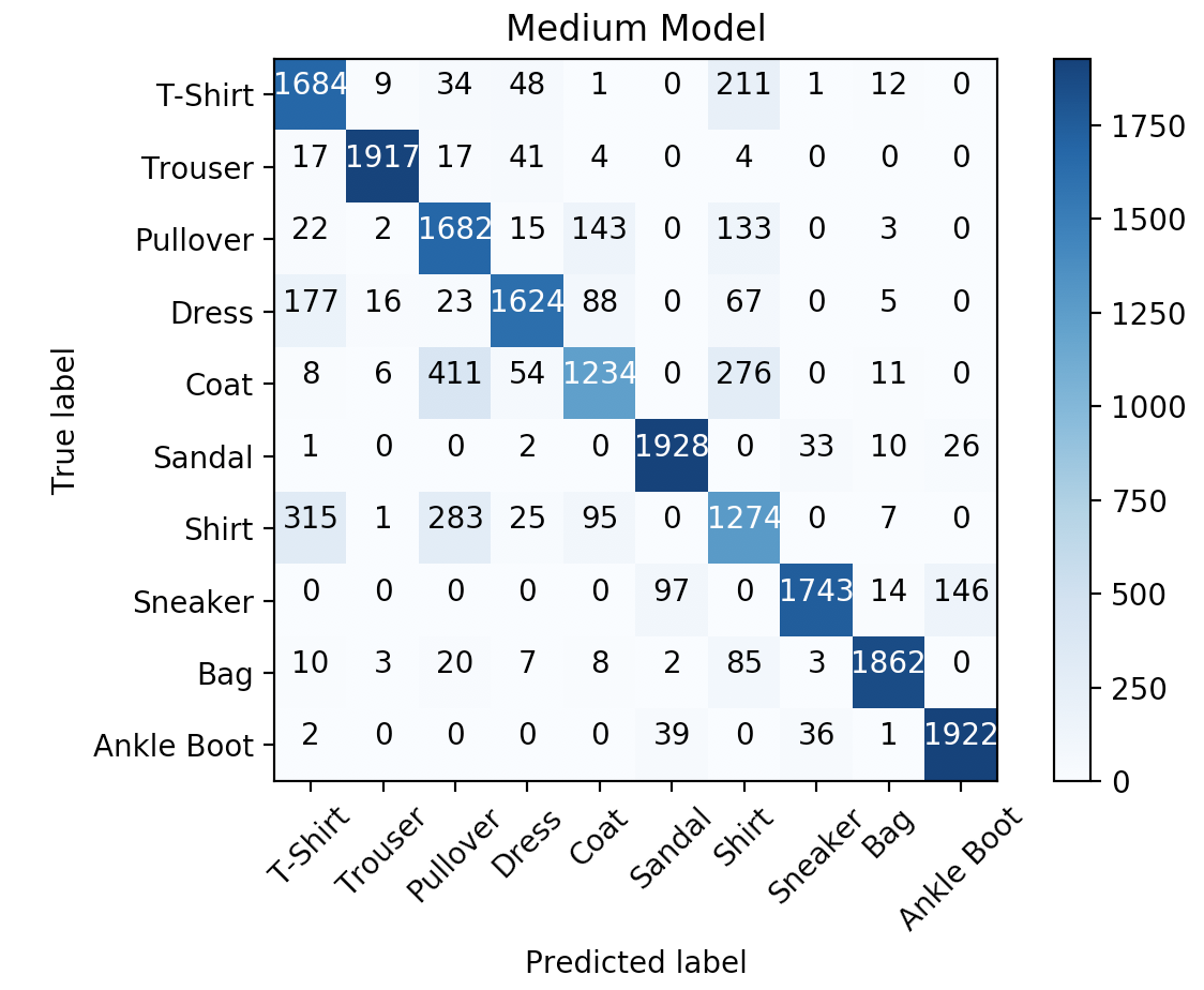
As before, we reserved multiple datasets for testing with the same distribution of labels as given in
dataset.csv. We will train and evaluate your model on our end using the sametrain()andevaluate()functions as given. Full points will be given for aMedium Modelfor num_epochs = 2, batch_size = 100, learning_rate = 0.001 if the accuracy on the reserved datasets and F1-Score is >= 82%. -
[15 pts] Advanced Model: In this part we ask you to fill in
__init__(self)andforward(self, x)of theAdvancedclass that is a subclass oftorch.nn.Module. We ask you to build a Convolutional Neural Network, which will consists of one or more convolutional layers (torch.nn.Conv2d) connected by the linear layers. The architecture is open-ended, so it is up to you to decide the number of layers, kernel size, activation functions etc. You can see performance of different architectures for this dataset here. The input to this model, unlike the input forEasyandMediumModels is expected to be different, and this is the reason why we asked you to reshape the images in Part 2.1. The output of this model remains the same as before.Once you have filled in
__init__(self)andforward(self, x)of theEasyModelclass you can use the following to see the performance of your>>> class_names = ['T-Shirt', 'Trouser', 'Pullover', 'Dress', 'Coat', 'Sandal', 'Shirt', 'Sneaker', 'Bag', 'Ankle Boot'] >>> num_epochs = 2 >>> batch_size = 100 >>> learning_rate = 0.001 >>> data_loader_reshaped = torch.utils.data.DataLoader(dataset=FashionMNISTDataset('dataset.csv', True), batch_size=batch_size, shuffle=True) >>> advanced_model = AdvancedModel() >>> train(advanced_model, data_loader_reshaped, num_epochs, learning_rate) >>> y_true_advanced, y_pred_advanced = evaluate(advanced_model, data_loader_reshaped) Epoch : 0/2, Iteration : 49/200, Loss: 0.7043, Train Accuracy: 80.2100, Train F1 Score: 79.9030 Epoch : 0/2, Iteration : 99/200, Loss: 0.4304, Train Accuracy: 84.0650, Train F1 Score: 83.9004 Epoch : 0/2, Iteration : 149/200, Loss: 0.4911, Train Accuracy: 85.0850, Train F1 Score: 84.4854 Epoch : 0/2, Iteration : 199/200, Loss: 0.3728, Train Accuracy: 86.9900, Train F1 Score: 86.9663 Epoch : 1/2, Iteration : 49/200, Loss: 0.3628, Train Accuracy: 87.2150, Train F1 Score: 86.9041 Epoch : 1/2, Iteration : 99/200, Loss: 0.3961, Train Accuracy: 87.7100, Train F1 Score: 87.7028 Epoch : 1/2, Iteration : 149/200, Loss: 0.3038, Train Accuracy: 88.9200, Train F1 Score: 88.9186 Epoch : 1/2, Iteration : 199/200, Loss: 0.3445, Train Accuracy: 89.2500, Train F1 Score: 88.8764 >>> print(f'Advanced Model: ' f'Final Train Accuracy: {100.* accuracy_score(y_true_advanced, y_pred_advanced):.4f},', f'Final F1 Score: {100.* f1_score(y_true_advanced, y_pred_advanced, average="weighted"):.4f}') Advanced Model: Final Train Accuracy: 89.2500, Final F1 Score: 88.8764 plot_confusion_matrix(confusion_matrix(y_true_advanced, y_pred_advanced), class_names, 'Advanced Model')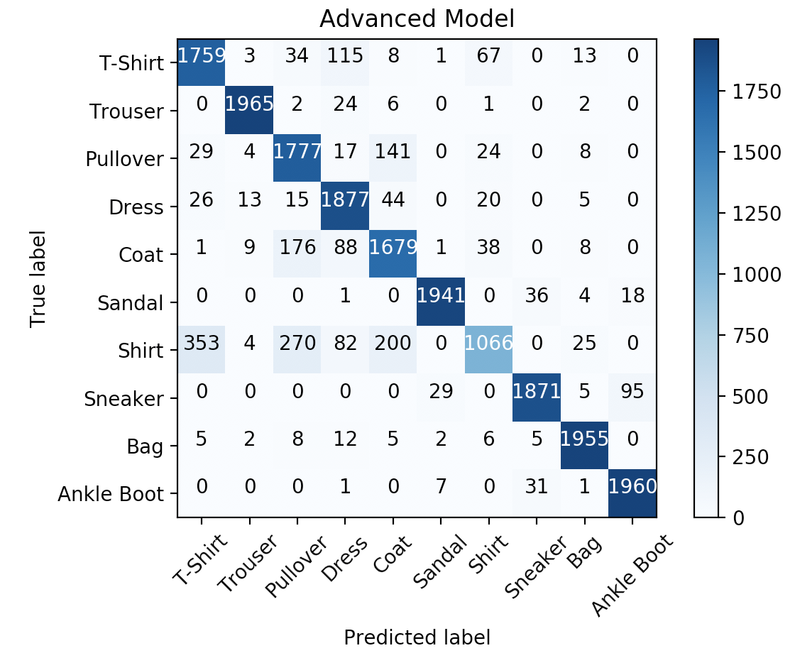
As before, we reserved multiple datasets for testing with the same distribution of labels as given in
dataset.csv. We will train and evaluate your model on our end using the sametrain()andevaluate()functions as given. Full points will be given for aAdvanced Modelfor num_epochs = 2, batch_size = 100, learning_rate = 0.001 if the accuracy on the reserved datasets and F1-Score is >= 88%.
- The
3. Feedback [5 points]
-
[1 points] What were the two classes that one of your models confused the most?
-
[1 points] Describe your architecture for the Advanced Model.
-
[1 point] Approximately how many hours did you spend on this assignment?
-
[1 point] Which aspects of this assignment did you find most challenging? Were there any significant stumbling blocks?
-
[1 point] Which aspects of this assignment did you like? Is there anything you would have changed?